
This blog post is about VICReg: Variance-Invariance-Covariance Regularization for Self-Supervised Learning, a 2021 paper by Adrien Bardes, Jean Ponce, and Yann LeCun that features prominently in LeCun’s recent vision to make human-like AI.
Our GitHub repo self_supervised now includes a validated implementation of VICReg (along with many of our other favorite methods like SimCLR, MoCo, and BYOL) and is very simple to set up. We also provide a simple Colab notebook with our VICReg implementation running so that you can start experimenting today.
Here, we present a friendly tutorial on self-supervised learning with VICReg, digging into the intuitions underlying the equations through explanations, visualizations, and code snippets.
Introduction
Self-supervised learning leverages unlabeled data to learn meaningful representations that can be adapted to a variety of downstream tasks. VICReg is the latest in a progression of self-supervised methods for image representation learning. Notable precursors include SimCLR, MoCo, BYOL, and SimSiam, each of which strives to eliminate or replace something that was previously thought necessary. VICReg continues in this vein, presenting a model that supplants all previous tricks with two statistics-based regularization terms on top of a simple invariance-preserving loss function.
If you’re new to self-supervised representation learning in computer vision, don’t worry; this post includes brief background and related work sections to get you up to speed.
If you’re already familiar with other self-supervised methods, feel free to skip ahead to the section titled “VICReg.”
Background
Traditional machine learning is mostly supervised, meaning that it’s trained on “ground truth” output labels for each input. Self-supervised learning automatically generates those output labels directly from the input data. For example, many modern language models like BERT are trained to guess the missing words that have been masked from raw text data. One obvious advantage of self-supervised learning is that it enables training without requiring humans to generate output labels by hand.
Self-supervised methods have recently gained traction in computer vision, where the state-of-the-art was previously dominated by supervised learning on datasets like ImageNet. The key insight underpinning these new methods is simple: input images that are similar according to a human should be similar according to the model. By augmenting an image in some semantics-preserving way (meaning the pixel values are not necessarily the same, but a human would still register them as being versions of the same image) we can generate pairs of images that should be encoded as similar vectors by the model.
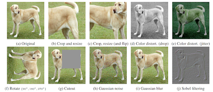
In detail, an input image is augmented to create two versions, and . This augmentation is often some combination of random crops, re-orientations, color perturbations, and noise injections. The two versions form a positive pair, with the loss function seeking to maximize the similarity of their representations. In some cases, the loss function simultaneously seeks to minimize the similarity of negative pairs—i.e. all other pairs—either directly or indirectly. Architecturally, the two versions of the image go through two networks whose weights are usually shared (“Siamese networks”) for at least some parts of the architecture.
The main challenge with Siamese networks is that there is a trivial solution: the two branches can learn to produce constant and identical output vectors, thereby satisfying the similarity condition without ever learning anything useful. This is often referred to as “mode collapse.” Approaches to avoiding mode collapse fall into two main camps, discussed in the next section.
Previous Work
Here we recap some of the most well-known prior works in self-supervised image representation learning and how they address the mode collapse problem. For a more exhaustive literature review, see e.g. Section 2 of the VICReg paper.
Explicitly contrastive methods: In these methods, mode collapse is avoided by including a repulsive term in the loss function that pushes negative pairs away from each other. Popular models SimCLR and MoCo mainly differ from one another in how they handle the need for a large number of negative pairs; SimCLR requires a large batch size, whereas MoCo maintains a memory bank of negatives from past batches. There is also SwAV, which does contrastive learning on the scale of clusters rather than individual images, i.e. simultaneously clustering the data while enforcing that different views of the same image are assigned to the same cluster.
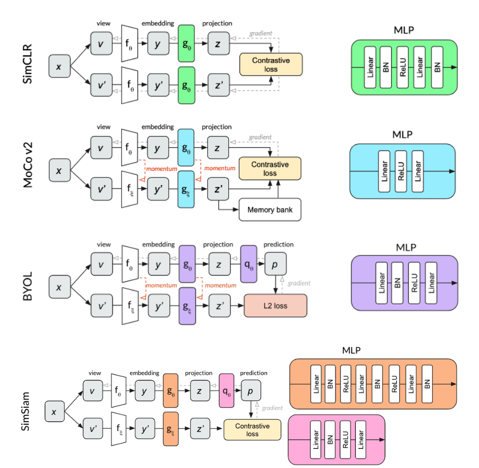
Asymmetric network methods: These methods don’t explicitly contrast negative pairs, but they avoid mode collapse by incorporating architectural tricks that introduce some asymmetry between the twins of the Siamese networks. BYOL continues a key idea from MoCo, in which the weights of one branch (momentum branch) are updated based on an exponential moving average of the weights of the other (online branch). However, BYOL also adds a prediction head to the online branch, showing that this removes the need for contrastive loss altogether. SimSiam takes things a step further, showing that momentum is not needed either—just the predictor and a stop-gradient to keep the backprop flowing through the online branch only. Since these methods do not rely on a large batch size or memory queue, they are more efficient, not to mention conceptually simple. However, how they avoid mode collapse is not fully understood, and both seem to critically require normalization. (To learn more about BYOL and our intuitions about how it uses batch norm, check out our other blog post.)
VICReg additionally takes inspiration from Barlow Twins, where the objective function drives the cross-correlation matrix of representations produced by the two branches towards the identity matrix. This captures the attraction between positive pairs and the repulsion between negative pairs while also decreasing redundancy between the different components of the vectors.
VICReg
High-Level Conceptual Description
VICReg has the same basic architecture as its predecessors; augmented positive pairs are fed into Siamese encoders that produce representations which are then passed into Siamese projectors that return projections .
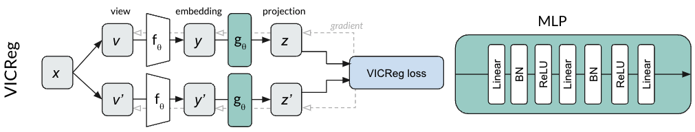
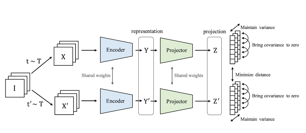
However, unlike its predecessors, the model requires none of the following: negative examples, momentum encoders, asymmetric mechanisms in the architecture, stop-gradients, predictors, or even normalization of the projector outputs. Instead, the heavy lifting is done by VICReg’s objective function, which contains three main terms: a variance term, an invariance term, and a covariance term.
Let’s break down each piece conceptually:
-
Variance. This regularization term constrains the variance along the batch dimension to be above some threshold for every embedding dimension, explicitly discouraging mode collapse.
-
Invariance. This term is the primary objective. Since the fundamental principle is that the representations produced by the model should be invariant to semantics-preserving data augmentations, the objective is a similarity metric to be minimized between positive pairs. However, this metric is not explicitly contrastive and thus does not require negative pairs or momentum.
-
Covariance. This regularization term forces the covariance matrix of the embeddings to be as close to diagonal as possible, encouraging the model to spread information across its embedding dimensions. In other words, it discourages dimension collapse.
Math and Pseudocode Description
Now that we understand the method conceptually, we can dig into the math. If you’re someone who thinks better in code, we also include actual snippets from our PyTorch implementation.
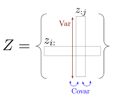
In the equations below, let be the matrix representing a batch, where and are the batch size and embedding dimension, respectively. Let be the th vector in the batch and let be a vector composed of the th element of each vector in the batch.
Variance
The variance term captures the variance of each embedding variable over a batch:
where is the target value for the standard deviation (they choose ), and is a small scalar put in place to prevent numerical instabilities (they choose ).
Notice that minimizing means forcing the batch-wise standard deviation to be above . As soon as this target is achieved, bottoms out at . A hinge function is used here because the point is not to encourage ever-increasing variance; higher variance isn’t necessarily better, it just needs to be above a certain threshold to avoid catastrophic failure i.e. mode collapse.
In PyTorch code:
# variance lossstd_z_a = torch.sqrt(z_a.var(dim=0) + self.hparams.variance_loss_epsilon)std_z_b = torch.sqrt(z_b.var(dim=0) + self.hparams.variance_loss_epsilon)loss_v_a = torch.mean(F.relu(1 - std_z_a))loss_v_b = torch.mean(F.relu(1 - std_z_b))loss_var = loss_v_a + loss_v_b
Invariance
The invariance term captures the invariance between positive pairs of embedding vectors:
This is just a simple mean-squared Euclidean distance metric. Notably, the vectors are un-normalized. In the paper, the authors do some experiments using the cosine similarity metric of SimSiam (which has the effect of projecting the vectors onto the unit sphere) instead. They find that performance drops a bit with this type of loss term, and argue that it’s too restrictive, especially since their covariance regularization term already prevents dimension collapse.
In PyTorch code:
# invariance lossloss_inv = F.mse_loss(z_a, z_b)
Covariance
The covariance term captures the covariance between pairs of embedding dimensions:
This one can be a bit tough to wrap your mind around dimensionally. Note that and are both vectors of length , resulting in covariance matrix . Whereas returns a number for each column vector , returns a number for the covariance between the centered versions of and . Minimizing means minimizing the off-diagonal components of the covariance matrix between centered embedding variables.
In PyTorch code:
# covariance lossN, D = z_a.shapez_a = z_a - z_a.mean(dim=0)z_b = z_b - z_b.mean(dim=0)cov_z_a = ((z_a.T @ z_a) / (N - 1)).square() # DxDcov_z_b = ((z_b.T @ z_b) / (N - 1)).square() # DxDloss_c_a = (cov_z_a.sum() - cov_z_a.diagonal().sum()) / Dloss_c_b = (cov_z_b.sum() - cov_z_b.diagonal().sum()) / Dloss_cov = loss_c_a + loss_c_b
Combined Loss Function
The loss function is a weighted combination of these three terms:
where are hyper-parameters (set to in the paper for the baseline) and the summations are over images and augmentations .
In PyTorch code:
weighted_inv = loss_inv * self.hparams.invariance_loss_weightweighted_var = loss_var * self.hparams.variance_loss_weightweighted_cov = loss_cov * self.hparams.covariance_loss_weightloss = weighted_inv + weighted_var + weighted_cov
That’s it! Thanks to this three-piece loss function with its variance and covariance regularization terms, VICReg avoids the need for negative pairs, momentum encoders, stop-gradients, predictors, or even batch norm layers.
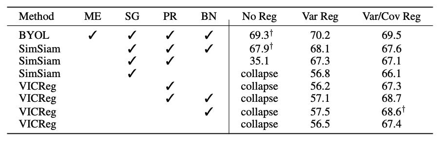
As the table above shows, these simple regularization terms prevent VICReg from collapsing even in the absence of the architectural elements required by other models. Indeed, the variance term alone is sufficient to prevent mode collapse, although the covariance term further boosts performance. Additionally, we see that these regulatization terms can be used to marginally improve the performance of other methods, or to save them from mode collapse when they are stripped of some of their previously critical components.
Learn More
If you found this tutorial interesting, you might enjoy reading the original paper or playing with our PyTorch implementation (which is also running in this simple Colab).
And, as always, we’re hiring! You can see our open roles here.
Thank you to teammates Josh Albrecht, Bartosz Wróblewski, Bryden Fogelman, and Abe Fetterman for feedback on the blog post and debugging help.